目录
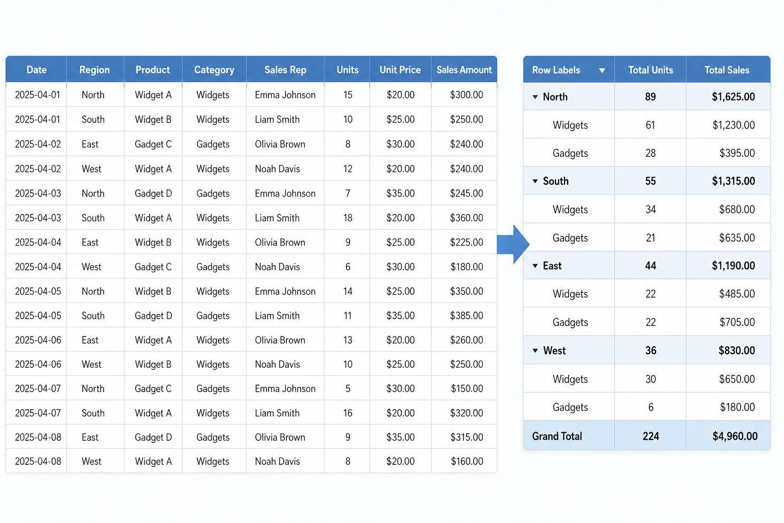
To create a PivotTable in WPS Spreadsheets, first organize your source data as one continuous list with clear column headers. Select the data range, choose Insert > PivotTable, decide whether the report should go in a new or existing worksheet, and then place fields into Rows, Columns, Values, and Filters. The layout can be changed later without altering the original data.
What a PivotTable helps you do
A PivotTable turns a detailed data list into a compact summary. Instead of manually adding formulas for every category, you can group records by fields such as department, product, month, or region, then summarize a numeric field such as revenue, quantity, or cost.
Use it when the same question can be viewed from several angles—for example, total sales by product, sales by region, or sales for one selected month.
Before you create the PivotTable
Clean source data is the foundation of a useful report. Keep one header row, use a meaningful heading for every column, and make sure each row represents one record. Avoid merged cells, blank header cells, and subtotal rows inside the source range, because they can make fields harder to interpret.
- Use one row for each transaction, item, or record.
- Put category information in separate columns, such as Date, Region, Product, and Sales.
- Keep amounts as numbers rather than number-looking text.
- Remove duplicate records when a record should be counted only once. See how to filter duplicate data in WPS Spreadsheets before building the report.
- Use consistent entries, such as “East” rather than a mixture of “East”, “east”, and “E”. For controlled input in future rows, see this WPS Spreadsheet data validation guide.
Create a PivotTable step by step
1. Select the source data
Click any cell in the data list or select the full range you want to summarize. Include the header row, because these headings become the field names in the PivotTable panel.
2. Insert the PivotTable
In WPS Spreadsheets, choose Insert > PivotTable. In the Create PivotTable dialog, check that the selected range includes all required columns and records.
3. Choose where the report should appear
Select New Worksheet when you want to keep the report separate from the raw data. Choose an existing worksheet only when you have a clear empty area for the report. Confirm the choice to create an empty PivotTable layout.
4. Build the report with the four field areas
Drag the available source fields into the areas in the PivotTable panel. The position of a field determines how the report is structured.
| Field area | Use it for | Example |
|---|---|---|
| Rows | Labels listed vertically | Product |
| Columns | Headings shown across the report | Region |
| Values | Numbers to summarize | Sum of Sales |
| Filters | A report-wide selection | Month |
As a general rule, place text categories in Rows, Columns, or Filters, and place numeric measures in Values. You can drag a field to another area at any time to view the same data differently.
5. Check the result
Confirm that the report answers the intended question. If the report should show total sales by product and region, Product can go in Rows, Region in Columns, and Sales in Values. Add Month to Filters if you need to switch the whole report between months.
Example: summarize sales by product and region
Example scenario: Imagine a worksheet with four columns: Date, Region, Product, and Sales. To see which products perform best in each region, put Product in Rows, Region in Columns, and Sales in Values. The resulting PivotTable displays a cross-tab summary, so you can compare totals without editing the original transaction list.
If you later need a visual summary, create a chart from the prepared report or data using this guide to make charts in WPS Spreadsheets. A chart is usually easier to read after the PivotTable has reduced a long source list into clear categories.
When the numbers look wrong
Values show Count instead of Sum
This commonly means WPS is treating the source entries as text rather than numbers, or the field contains blanks and mixed values. Review the source column, convert number-looking entries to real numbers, and then recreate or adjust the summary as needed.
A new row is missing from the report
Check whether the new row is inside the source range used when the PivotTable was created. If it falls outside that range, expand or redefine the source range before updating the report. Also make sure the new row uses the same headers and data format as the existing list.
The field list has confusing or blank names
Return to the source data and inspect the header row. Every column should have one nonblank, distinct heading. Rename duplicate or empty headers, then create the PivotTable again.
Totals seem too high
Look for repeated records, repeated imported rows, or multiple entries that should not be added together. Filter the source list first to inspect the underlying records, then rebuild the report if necessary.
Verification status and usage notes
This article is compiled from relevant official help materials from the brand. Specific feature locations, rule names, and available styles may vary by system, region, account, and version; use the current client or official page as the reference. This is a third-party usage tutorial, not an official help page from the relevant brand.
FAQ
Do I need to select the whole table before creating a PivotTable?
Select the complete source range, including its header row. If your data is one continuous list, clicking a cell within the list may also allow WPS to identify the range, but checking the range in the creation dialog is still important.
Can I change Rows and Columns after creating the report?
Yes. Move fields between Rows, Columns, Values, and Filters to create a different view of the same source data.
Should I create the PivotTable on a new worksheet?
For most beginners, a new worksheet is the clearer choice because it separates the report from the editable source data.
Why should I use Filters in a PivotTable?
Filters let you limit the entire report to one selected category, such as a month, region, or department, while keeping the underlying data unchanged.